Tempo
The term tempo in the context of audio and music refers to the speed or pace of a piece of music. It’s a fundamental characteristic of music, and it’s often measured in beats per minute (BPM).
In the context of audio data analysis with Librosa, when we estimate tempo, we are using mathematical techniques to figure out how fast or slow a piece of music is without having to listen and count the beats ourselves. For example, to extract the tempo of the audio, you can use the following code:
import librosa
import librosa.display
import matplotlib.pyplot as plt
Load an audio file
audio_file = “cat_1.wav”
y, sr = librosa.load(audio_file)
Extract the tempo
tempo, _ = librosa.beat.beat_track(y=y, sr=sr)
print(f”Tempo: {tempo} BPM”)
Output:
Tempo: 89.10290948275862 BPM
This code utilizes librosa.beat.beat_track() to estimate the tempo of the audio.
Application: Music genre classification.
Example: Determining the tempo of a music track can help classify it into genres. Fast tempos might indicate genres such as rock or dance, while slower tempos could suggest classical or ambient genres.
Chroma features
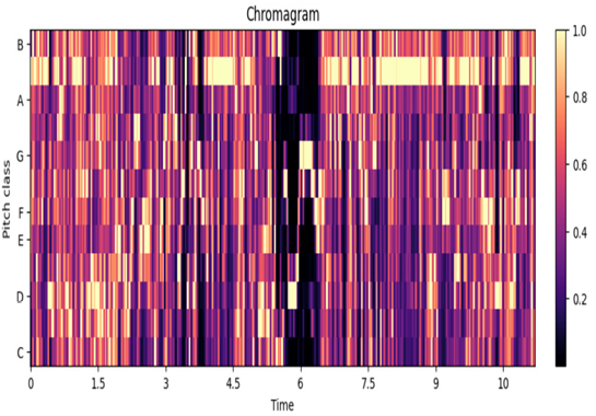
Chroma features represent the energy distribution of pitch classes (notes) in an audio signal. This can help us identify the musical key or tonal content of a piece of music. Let’s calculate the chroma feature for our audio:
Calculate chroma feature
chroma = librosa.feature.chroma_stft(y=y, sr=sr)
Display the chromagram
plt.figure(figsize=(12, 4))
librosa.display.specshow(chroma, y_axis=’chroma’, x_axis=’time’)
plt.title(“Chromagram”)
plt.colorbar()
plt.show()
Here’s the output:

Figure 10.2 –A chromagram
In this code, librosa.feature.chroma_stft() is used to compute the chroma feature, and librosa.display.specshow() displays it.
Application: Chord recognition in music.
Example: Chroma features represent the 12 different pitch classes. Analyzing chroma features can help identify chords in a musical piece, aiding in tasks such as automatic chord transcription.
Mel-frequency cepstral coefficients (MFCCs)
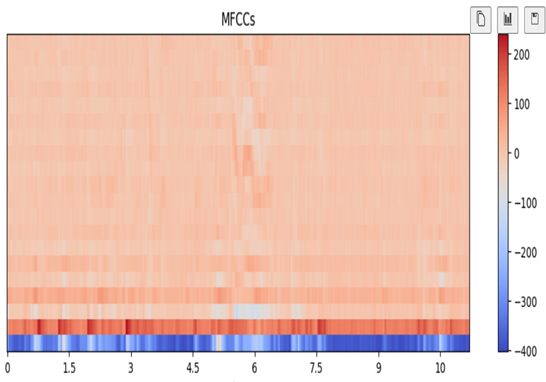
MFCCs are a widely used feature for audio analysis. It captures the spectral characteristics of an audio signal. In speech and music analysis, MFCCs are commonly used for tasks such as speech recognition. Here’s how you can compute and visualize MFCCs:
Calculate MFCC
mfccs = librosa.feature.mfcc(y=y, sr=sr)
Display the MFCCs
plt.figure(figsize=(12, 4))
librosa.display.specshow(mfccs, x_axis=’time’)
plt.title(“MFCCs”)
plt.colorbar()
plt.show()
Here is the output:

Figure 10.3 – Plotting MFCCs
librosa.feature.mfcc() calculates the MFCCs, and librosa.display.specshow() displays the MFCCs.
Application: Speech recognition.
Example: Extracting MFCCs from audio signals is common in speech recognition. The unique representation of spectral features in MFCCs helps us identify spoken words or phrases.